STATegra EMS: The data structure
The overall objective of the STATegra EMS is to serve as a logbook for high-throughput genomics projects performed at research labs by providing an easy-to-use tool for the annotation of experimental design, samples, measurements, and the analysis pipelines applied to the data. Experimental data and metadata are organized in the EMS around three major metadata modules (Figure 2): the Experiment module that records experimental design information and associated samples; the Samples module that collects all information on the used biomaterial; and the Analysis module that contains analysis pipelines and results. Both Sample and Analysis modules have been defined broadly to accommodate data from different type of omics experiments and still provide a common annotation framework. Commonly used standards in omics experimental data annotations were used when defining data specifications to facilitate EMS interoperability. In particular, we leveraged MIAPE [16] for proteomics analysis annotation, metabolomics guidelines proposed by [17] and [18] and MIAME [19] and MINSEQE [20] for sequencing experiments.

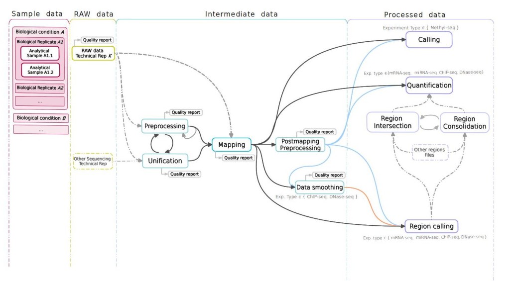
Figure 1 Metadata Module structure in STATegra EMS. The Sample module stores information of biological conditions, biological replicates and the associated analytical samples. The analysis module contains all analysis steps from raw to processed data. Both samples and analyses are associated to one or more experiments within the Experiment module.
Sample and Analysis modules contain distinct Information Units (IUs), which are the basic elements of data input into the system and are connected by an experimental or analysis workflow. The Experiment Module is a wrapper of Samples and Analyses with one single data input form.
-
Experiment module: The experiment is the central unit of information of the STATegra EMS. An Experiment is defined by some scientific goals and a given experimental design that addresses these goals. This design implies a number of biological samples and an array of omics measurements, which are assigned to the Experiment.
-
Sample module. This section hosts the information about biological conditions and their associated biological replicates and analytical samples. The IUs of this module are:
Biological Condition. These are defined by the experimental design and consist of a given biological material such as the organism, cell type, tissue, etc. and, when applicable, an experimental condition such as treatment, dose or time-point for time-series samples.
Biological Replicate. Each Biological Condition is assessed by using one or more biological replicates that may or may not correspond to the same experimental batch. The Biological Replicate stems directly from Biological Condition by adding a replicate number and, if applicable, a batch number.
Experimental Batch. Frequently, when an experiment is composed of a large number of samples, only some of them can be generated at the same time. These samples correspond to the same batch. Batch information is relevant to identify systematic sources of noise that might affect all samples within the batch.
Analytical Sample. Omics experiments analyze molecular components of biological samples using a given experimental protocol with the resulting analytical sample ready-to-be-measured by the high-throughout techniques. For example, a RNA-seq analytical sample is obtained after using a cytosolic mRNA extraction protocol. Similarly for metabolomics, different analytical samples can be obtained by applying multiple extraction protocols that target distinct metabolic compounds.
-
Analysis module. The Analysis module stores high-throughput molecular data obtained by the omics technologies and the data generated after processing of the primary raw data files. In contrast to the Sample module where only metadata is stored, the Analysis module also stores pointers to data files. The Analysis module consists of three data and one logical IUs:
Raw Data. These files contain the data as produced by the omics equipment. For example, fastq files in the case of sequencing experiments and NMR .raw files in the case of metabolomics experiments. The Raw data IU also contains detailed information of the experimental protocol applied to the analytical sample, i.e., the library preparation protocol followed in a RNA-seq experiment or the NMR analysis characteristics in the case of metabolomics.
Intermediate Data. This IU covers all processing steps from raw data to process data. Different omics experiment might require zero, one, or several intermediate steps. For example, in the case of RNA-seq, the mapping to a reference genome that produces a bam file constitutes an intermediate step. ChIP-seq will generally have two intermediate steps consisting of read mapping and peak calling.
Processed Data. The Processed data IU contains the final processing step that result in a data file containing the final signal values for the omics assay.
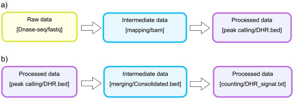
Analysis. The STATegra EMS includes an additional IU, the Analysis, which is constructed by connecting some of the previous data IUs to define a data processing workflow. Figure 3 shows a generic representation of the workflow elements used in sequencing data analyses. An Analysis will start on a raw data file obtained from a particular analytical sample, continue through one or several intermediate data files covering different processing steps (such as trimming, mapping, filtering, merging, etc), and finalize in a processed data file that contain the signal values of the omics features. Alternatively, an Analysis can take as input a processed data file and apply additional processing steps to render a higher-level processed data. For example, in DNase-seq analysis, a primary workflow would be to call DNase hypersensitivity regions (DHR) by applying a peak-calling algorithm to a BAM file of mapped reads (Figure 4 A); whereas a secondary Analysis could involve merging DHR.bed files from N different samples to obtain a set of consolidated regions and then counting the number of reads of each sample in the consolidated region set to generate a per-sample signal value file (Figure 4 B).
In terms of data consistency, a unique Analysis ID is always associated to one Processed Data ID and describes the set of steps involved in obtaining that particular processed data. Moreover, an Analysis is always associated to one or more Experiments and, since the Analysis workflow can be traced back to raw data and its associated analytical samples, the Analysis provides the link between the Experiment and the Sample modules. By default, when a new Analysis is created, it will be assigned to the currently active Experiment. Figure 5 shows the data input window at the Analysis module. The central panel displays the input form for the different analysis steps, while at the bottom a graphical representation of the workflow allows easily monitoring the elements and structure of the Analysis.

Figure 2. STATegra EMS analysis workflow components. The workflow is linked to an analytical sample object and consists of raw, intermediate and processed data IUs.

Figure 3. Example of primary and secondary workflow for a DNase-seq analysis. Primary workflow (a) involves calling DNase hypersensitivity regions (DHR) by applying a peak-calling algorithm to a BAM file of mapped reads whereas secondary workflow (b) involves merging of DHR.bed files from different samples to obtain a set of consolidated regions and then counting the number of reads of each sample in the consolidated region set to generate a per-sample signal value file.